Building Data History in Databricks: A Custom Strategy as an Alternative to DLT

In today’s data-driven world, having a reliable strategy to track and manage historical data is more than a technical necessity — it’s a competitive advantage. But what happens when you cannot or choose not to use tools like Databricks DLT? In this blog, we will dive into a custom strategy, optimised for efficiency and aligned with the Medallion Architecture. Get ready to explore a scalable, transparent approach that simplifies data versioning, enhances lineage, and unlocks the full potential of your data ecosystem!

Data, requirements and why history matters

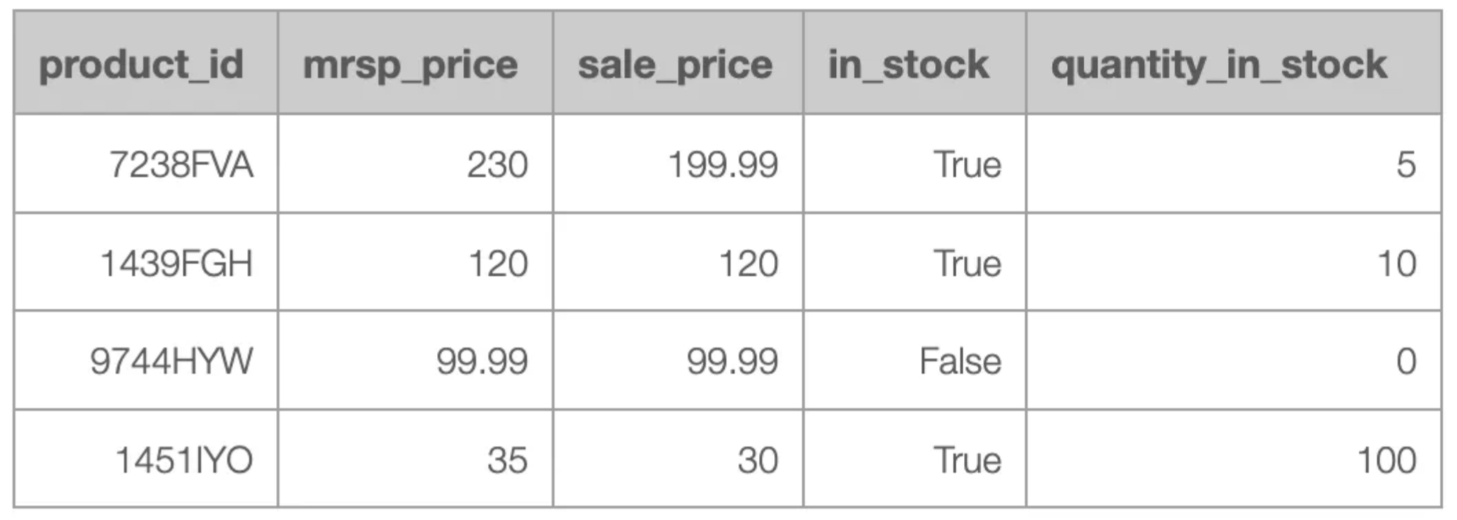
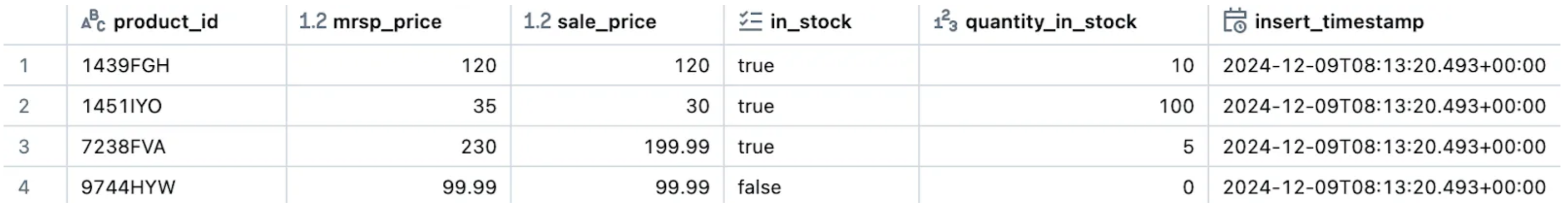
To set the stage, we are addressing a task for a retail company that sells products through its e-shop. Currently, their data only reflects the present state, as no historical records are preserved. As part of their digital transformation strategy, the company has decided to retain historical changes. Additionally, they plan to migrate their data to a cloud provider and leverage Databricks for data processing. Their existing data infrastructure follows a star schema architecture, with data accessible through an exposed API. The goal is to enable straightforward access to both historical data and the current state. For simplicity, we will focus on a single dimension of the star schema, extracted via the API. A sample of this dimension is as follows:

Maintaining accurate historical data is essential for compliance, informed decision-making, and operational resilience. Many industries require detailed records to meet regulatory standards, facilitate audits, and ensure data integrity. Beyond compliance, historical data enables root cause analysis, supports advanced analytics, and drives data-driven forecasts by revealing trends and patterns. It also strengthens operational resilience, aiding disaster recovery and rollbacks to stable versions. Reliable data history fosters trust, transparency, and collaboration, empowering teams with consistent records. Organisations that prioritise robust historical data are better prepared to meet compliance demands, navigate complexities, and fully leverage their data’s potential.

Techniques to track data history (SCD)

In database management and data warehousing, Slowly Changing Dimensions (SCD) play an essential role in preserving historical data and ensuring data integrity. SCDs are used to track changes in dimension attributes over time. These dimensions are especially valuable for tracking attributes that change infrequently or unpredictably over time. The concept of SCD provides a structured approach to handle such changes, ensuring historical records remain intact and accessible for analysis.

A dimensional table typically contains a primary key (or composite primary key) to uniquely identify each record, alongside other fields carrying important descriptive information known as dimensional data. The primary key serves as the link between dimension tables and fact tables, highlighting the need for robust models to handle both current and historical data. Data Architects have relied on the SCD framework for decades to design data warehouses, and the concept remains relevant in modern data architectures.

Main SCD types:

• SCD Type 1: The simplest to implement, this method overwrites existing records when changes occur. It does not maintain historical data and is suitable for scenarios where historical tracking is unnecessary or irrelevant.
• SCD Type 2: The most common approach, this type creates a new row for every change, preserving all historical versions of the record. By maintaining historical data, this approach supports auditing and trend analysis. In this approach, you identify history by adding a flag column to indicate the current active record or by using timestamp columns to track the “valid from” and “valid to” periods for each record.
• SCD Type 3: This approach tracks limited historical changes by maintaining previous versions in separate columns within the same record. It is useful when only a few historical versions need to be retained. While it consumes less storage and enables faster queries due to limited history, it does not provide a complete record of changes over time.
• SCD Type 4: This approach is very similar to SCD Type2. The difference is that here we have two tables. One with all the current data and one other with the historical data (only older records not the current).

What is available in Databricks (DLT) and restrictions

As Databricks describes, “Delta Live Tables (DLT) is a declarative ETL framework for the Databricks Data Intelligence Platform that helps data teams simplify streaming and batch ETL cost-effectively.” With DLT, users can define transformations and let the framework handle task orchestration, cluster management, monitoring, data quality enforcement, and error handling automatically. This makes it particularly attractive for data teams aiming to streamline workflows and focus on data insights.

DLT supports both SCD Type 1 and Type 2, making it straightforward to implement slowly changing dimensions. While Databricks offers extensive documentation to guide developers, one critical prerequisite is the structure of the source data. The source data must include metadata and be versioned through snapshots rather than being overwritten. These snapshots, timestamped either at the table or file level, provide a stable view of the data at a given time, enabling the management of temporal data and a clear historical record.

However, applying the DLT strategy directly may not always be feasible due to the constraints of the existing source. In such cases, the source data can be transformed and brought into Databricks in a suitable format, enabling DLT pipelines to perform CDC (perform cdc full table snapshots using DLT) with full table snapshots. At this stage, it’s crucial to evaluate whether to proceed with DLT or adopt a custom solution. While DLT offers powerful features and automation, it introduces potential vendor lock-in, as migrating pipelines to another platform in the future would require a complete rebuild. DLT compute is generally more expensive than normal job compute, and as such the end pipeline can end up more expensive. Balancing the trade-offs between functionality, cost, and portability will help determine the best approach for your specific requirements.

Proposed strategy

For the reasons mentioned above, our proposal is to adopt a custom solution tailored to our specific requirements. A key consideration for this approach is the need for our ingestion pipeline to perform a full scan of both old and new data during each run to identify updates, inserts, and deletes. While necessary, this process is both time-consuming and resource-intensive. Therefore, it is imperative that subsequent procedures are optimized for efficiency to minimise overall performance costs.

Following our requirements, we propose to follow a strategy that is a combination of SCD Type 2 and 4. It is very important at this point to highlight the fact that we propose an insert-only strategy. This means that each change, independent if it is an insert, update or delete will be treated as an insert. However, even within this framework, important decisions must be made, such as determining the additional columns required for versioning, how to signify changes in fields, and how to structure our tables and views to ensure clear differentiation between historical and current records.

To meet these needs, we propose adding three extra columns to the existing schema:

• insert_timestamp: Captures the exact time when a row was ingested into the system.
• is_deleted: A boolean field indicating whether a specific record has been marked as deleted.
• hash_key: A unique identifier for each record, generated using the SHA-256 hash function to ensure data integrity.Here, the business key is the input for the hash function.

As far as the data architecture is concerned, we propose the medallion architecture as it was introduced by Databricks.

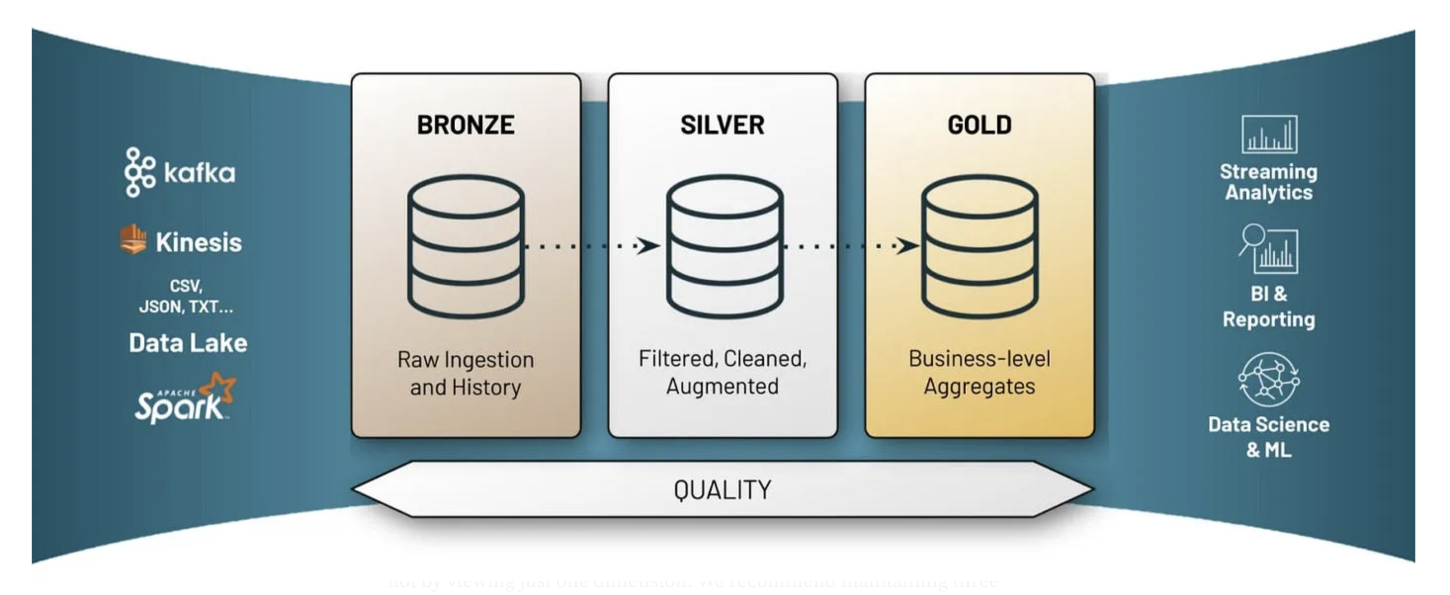
medallion-architecture-best-practices-for-managing-bronze-silver-and-gold

The Medallion Architecture (Databricks medallion architecture) is a robust design framework for structuring data workflows to ensure scalability, reliability, and performance. It organises data into three distinct layers — Bronze, Silver, and Gold — to streamline data ingestion, transformation, and analytics. The Bronze layer serves as the raw landing zone for all incoming data, capturing it in its original form for traceability. The Silver layer focuses on cleaning, enriching, and transforming the raw data into a refined state, making it ready for analysis or downstream consumption. Finally, the Gold layer provides highly curated datasets, optimized for specific business use cases such as reporting, machine learning, or advanced analytics. This layered approach promotes a clear separation of concerns, enabling teams to maintain data quality, track lineage, and cater to diverse business needs while handling large-scale, complex data ecosystems efficiently.

Of course, in order to understand and appreciate the medallion architecture someone needs to see the bigger picture and the complete data model and not by viewing just one dimension. We recommend maintaining three distinct tables: the raw table, the history table, and the current table. The raw table acts as the foundational layer (bronze), capturing unaltered ingested data, while the history and current tables (silver) work as unified and curated aspects of the source data. With that information available on the silver layer, business analysts can leverage them to create tables (gold) to cater their specific needs. By the proposed approach, we achieve several key benefits that will be presented later in this blog.

Implementation

At this section we will showcase a reproducible example of our proposed solution, with a simplified example focusing on the basic components.

Let’s import the libraries that we will need for our implementation.

from pyspark.sql.functions import col, sha2, lit, when, concat_ws
from datetime import datetime, timezone,timedelta
from pyspark.sql import SparkSession
from pyspark.sql.types import StructType, StructField, StringType, IntegerType,
                                    

In this showcase, we will use a set of well-structured and intuitive PySpark functions to demonstrate how to build and manage a product price and availability history system. Each function is designed with a clarity-first mindset, and includes detailed docstrings that provide all the necessary information. These functions cover a wide range of tasks, such as processing data with hash keys, identifying upserts(updates and inserts) and deletes, preparing records for insertion, and creating history and current state tables. By combining modularity and readability, this collection of functions offers an efficient and reusable foundation for managing slowly changing dimensions and tracking data changes over time.

def get_active_records_from_df(current_schema_table_name): 
   """ 
   Retrieve the 'active' records from the given table. 
   Parameters: 
   - current_schema_table_name: The catalog, schema and name of the table to be queried. 
   Returns: 
   - DataFrame with the active records. 
   """ 
       query = f""" SELECT * FROM {current_schema_table_name} ;""" 
   df_old = spark.sql(query) 
   return df_old 
 def add_prefix_to_column_names(df, prefix): 
   """ 
   Add a prefix to all column names of the DataFrame. 
   Parameters: 
   - df: Spark DataFrame. 
   - prefix: Prefix to be added to column names. 
   Returns: 
   - DataFrame with prefixed column names. 
   """ 
   for col_name in df.columns: 
       new_col_name = f"{prefix}{col_name}" 
       if new_col_name != col_name: 
           df = df.withColumnRenamed(col_name, new_col_name) 
   return df 
  def process_dataframe(df, current_timestamp, prefix=''): 
   """ 
   Process the given DataFrame by adding extra columns and hashing. The extra columns are: 
    insert_timestamp, is_deleted and hash_key 
   Parameters: 
   - df: Spark DataFrame to be processed. 
   - prefix: Optional prefix for column names. Default is an empty string. 
   - current_timestamp: Current timestamp to be used for insert_timestamp. 
   Returns: 
   - Processed Spark DataFrame. 
   """ 
   df = df.withColumn("all_columns", concat_ws('_', *df.columns)).withColumn(f"{prefix}hash_key", sha2(col("all_columns"), 256)).drop("all_columns") 
       # Add extra columns 
   df = df.withColumn(f"{prefix}insert_timestamp", lit(current_timestamp)) 
   df = df.withColumn(f"{prefix}is_deleted", lit(False)) 
   return df 
 def identify_upserts(df_new, df_old, hash_key_new, hash_key_old): 
   """ 
   Identify upserts by performing a left anti-join between df_new and df_old based on the hash key. 
   Parameters: 
   - df_new: Spark DataFrame containing new records. 
   - df_old: Spark DataFrame containing old records. 
   - hash_key_new: The hash key of df_new used for joining. 
   - hash_key_old: The hash key of df_old used for joining. 
   Returns: 
   - DataFrame containing records in df_new that are not present in df_old. 
   """ 
   upserts = df_new.join(df_old, df_new[hash_key_new] == df_old[hash_key_old], "left_anti") 
   return upserts 
 def identify_deletes(df_new,df_old,prefix_new,pkey): 
   """ 
    Identify deletes by performing a left anti-join between df_new and df_old based on the primary key. 
   Parameters: 
   - df_new: Spark DataFrame containing new records. 
   - df_old: Spark DataFrame containing old records. 
   - prefix_new: The prefix of the new dataframe. 
   - pkey: The primary key of the dataframe. 
   Returns: 
   - DataFrame containing records in df_old that are not present in df_new. 
   """ 
   join_condition = '' 
   join_condition = f'(df_new["{prefix_new}{pkey}"] == df_old["{pkey}"]) & ' 
   join_condition =join_condition[:-2] 
   join_condition_expr = eval(join_condition) 
   deletes = df_old.join(df_new, join_condition_expr, "left_anti") 
   if "sku" in df_old.columns: 
       deletes = deletes.filter(col("sku").isNotNull()) 
   return deletes 
 def prepare_rows_to_insert(upserts,deletes, prefix_new, current_timestamp): 
   """ 
   Prepare rows to insert by adding extra columns and hashing. The extra columns are: 
   insert_timestamp, is_deleted and hash_key 
   Parameters: 
   - upserts: Spark DataFrame containing records to be inserted. 
   - deletes: Spark DataFrame containing records to be deleted. 
   - prefix_new: The prefix of the new dataframe. 
   - current_timestamp: Current timestamp to be used for insert_timestamp. 
   Returns: 
   - Spark DataFrame containing rows to be inserted. 
   """ 
   deletes = deletes.withColumn("is_deleted", lit(True)) 
   deletes = deletes.withColumn("insert_timestamp", lit(current_timestamp)) 
   upserts = upserts.select([col(column).alias(column.replace(prefix_new, "")) for column in upserts.columns]) 
   df_to_insert = upserts.union(deletes) 
       return df_to_insert 
 def create_product_price_availability_history_table(): 
   """ 
   Create the history table for the product_price_availability table. 
   """ 
   query = f""" 
       CREATE OR REPLACE TABLE {raw_schema_table_name}_history AS 
           SELECT 
               product_id,mrsp_price,sale_price,in_stock,quantity_in_stock, 
               insert_timestamp AS valid_from, 
               CASE 
                WHEN is_deleted = True THEN insert_timestamp 
                ELSE LEAD(insert_timestamp) OVER ( 
                   PARTITION BY product_id 
                   ORDER BY insert_timestamp 
                   ) 
               END AS valid_to 
           FROM 
               {raw_schema_table_name}; 
   """ 
   spark.sql(query)
def create_product_price_availability_current_table(): 
   """ 
   Create the current table for the product_price_availability table. 
   """ 
   query = f""" 
       CREATE OR REPLACE TABLE {raw_schema_table_name}_current AS 
           SELECT 
                product_id,mrsp_price,sale_price,in_stock, 
               quantity_in_stock,insert_timestamp 
           FROM ( 
               SELECT *, ROW_NUMBER() OVER ( 
                   PARTITION BY product_id ORDER BY insert_timestamp DESC) AS row_num 
               FROM {raw_schema_table_name}            ) 
ranked 
           WHERE row_num = 1 AND NOT is_deleted; 
   """ 
   spark.sql(query)
                                    

For simplicity and for demo purposes, we will use predefined mock data to demonstrate the functionality of our PySpark functions. However, in a production environment, data would typically come from sources such as databases, APIs, or files. In such cases, additional code would be necessary to retrieve the raw data and transform it into the desired format before applying our proposed logic. While this example focuses on the core processing steps, it’s important to recognize that the initial data extraction and preparation are equally critical for achieving the final result.

spark = SparkSession.builder.getOrCreate()
# Define the schema
schema = StructType([ 
   StructField("product_id", StringType(), False), 
   StructField("mrsp_price", DoubleType(), True), 
   StructField("sale_price", DoubleType(), True), 
   StructField("in_stock", BooleanType(), True), 
   StructField("quantity_in_stock", IntegerType(), True)
])
# Data at "to" point of time
data_to = [ 
   ("7238FVA", 230.00, 199.99, True, 5), 
   ("1439FGH", 120.00, 120.00, True, 10), 
   ("9744HYW", 99.99, 99.99, False, 0 ), 
   ("1451IYO", 35.00, 30.00, True, 100)
]
# Data at "t1" point of time (1 addition, 1 delete, 1 update)
data_t1 = [ 
   ("5446HHJ", 18.00, 18.00, True, 10), 
   ("1439FGH", 120.00, 109.99, True, 10), 
   ("9744HYW", 99.99, 99.99, False, 0 ), 
   ("1451IYO", 35.00, 30.00, True, 100)
]
# Create the DataFrames for t0 & t1
df_to = spark.createDataFrame(data_to, schema)
df_t1 = spark.createDataFrame(data_t1, schema)
                                    

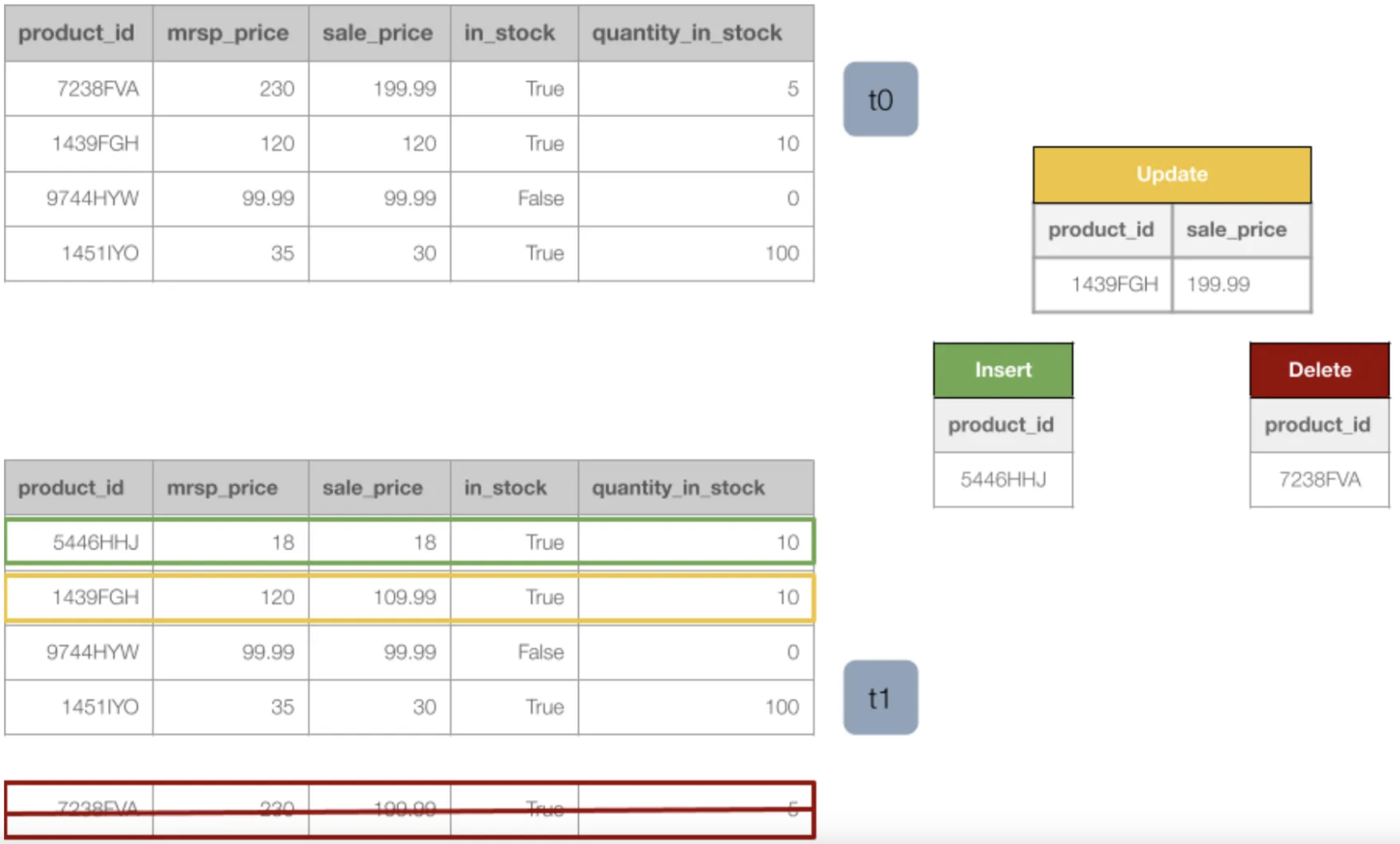
As it is easily depicted from the figure below, we have a dataframe with the initial data at time zero and we have another dataframe for the new version of the data. In the new version of the data we have 1 product that was not there before (insert), 1 product that is no longer there (delete) and 1 product that has a change in the sale_price field (update).

Let’s set now the configuration variables that we will need:

current_schema_table_name="hive_metastore.db_pna_sales.product_price_availability_current"
history_schema_table_name = "hive_metastore.db_pna_sales.product_price_availability_history"
raw_schema_table_name = "hive_metastore.db_pna_sales.product_price_availability"
pkey = "product_id"
                                    

The following snippet of code is needed only for the first execution, the first ingestion of data. Because before the first execution there is no data in our tables to compare with, when the new version of the data comes.

df_to = process_dataframe(df_to,current_timestamp)
df_to.write.format('delta').mode('overwrite').saveAsTable(raw_schema_table_name)
create_product_price_availability_history_table()
create_product_price_availability_current_table()
                                    

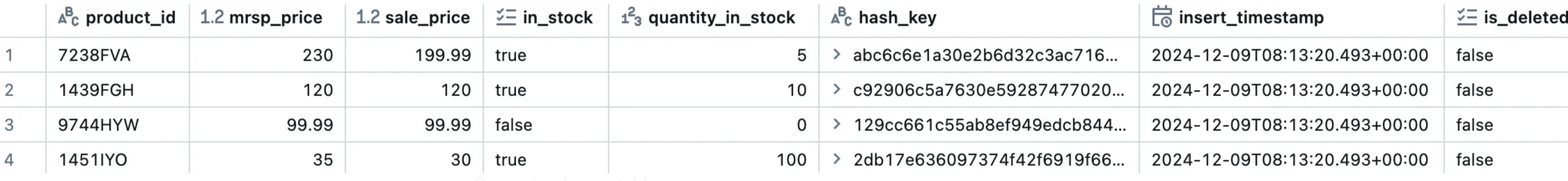
At this point we have our first version of the code! Let’s have a look at the three tables that have been created.

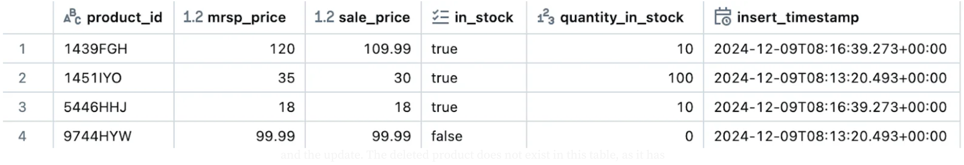
Raw_schema_table_name:

Current_schema_table_name:

History_schema_table_name:

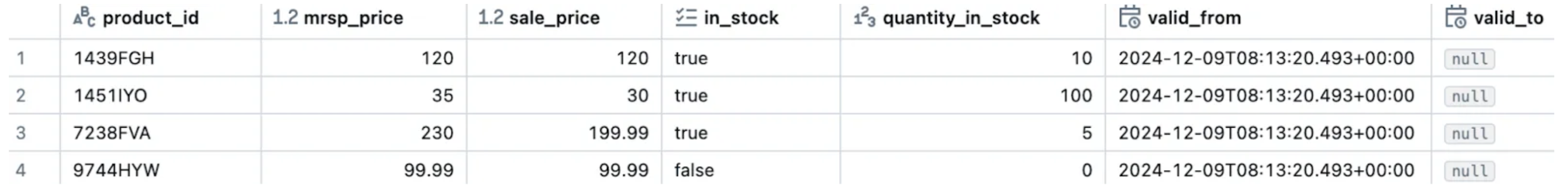
For the moment, our three tables are identical. This is expected as there has been only one ingestion run (t0). In the below snippet of code we demonstrate the ingestion pipeline that will update our three tables in the manner we want.

try: 
   df_t1 = spark.createDataFrame(data_t1, schema) 
   print("new data loaded") 
   df_old = get_active_records_from_df(raw_schema_table_name,pkey) 
   print("get_active_records_from_df finished") 
   df_t1 = add_prefix_to_column_names(df_t1,'new_') 
   current_timestamp = datetime.now(timezone.utc) 
   df_t1 = process_dataframe(df_t1,current_timestamp,'new_') 
   print("process_dataframe finished") 
   upserts = identify_upserts(df_t1, df_old, "new_hash_key", "hash_key") 
   upserts_count = upserts.count() 
   print(f"identify_upserts finished, upserts:{upserts_count}") 
   deletes = identify_deletes(df_t1, df_old, 'new_',pkey) 
   deletes_count = deletes.count() 
   print(f"identify_deletes finished, deletes:{deletes_count}") 
   df_to_insert = prepare_rows_to_insert(upserts,deletes, 'new_',current_timestamp)
df_to_insert.write.format('delta').mode('append').saveAsTable(raw_schema_table_name) 
   print("new rows inserted into table") 
   create_product_price_availability_history_table() 
     print("created history table") 
   create_product_price_availability_current_table() 
   print("created current table")
except Exception as e: 
   print(f"Error: {e}") 
   raise
                                    

Printed output:

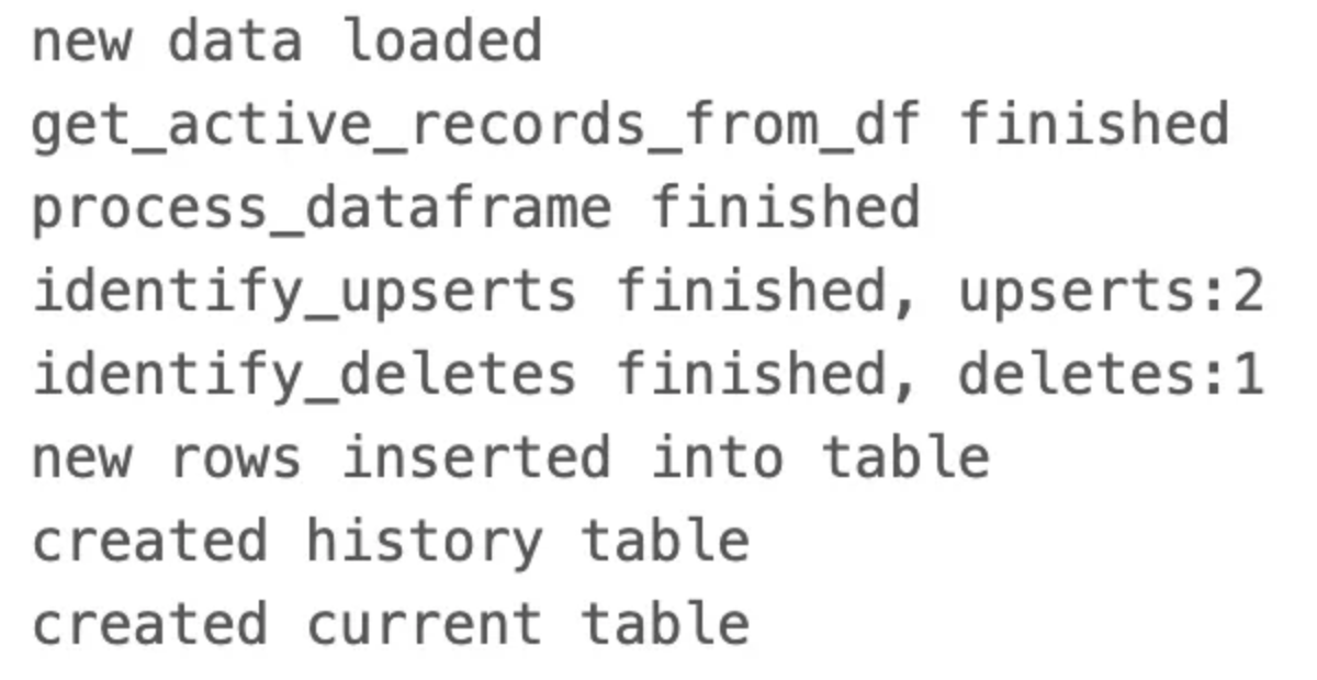
Our ingestion pipeline worked just fine. As it can be illustrated there are 2 identified upserts (1 insert and 1 update) as well as 1 identified delete, as expected. By having a look at the refreshed tables we can easily obtain whatever information needed from each table.

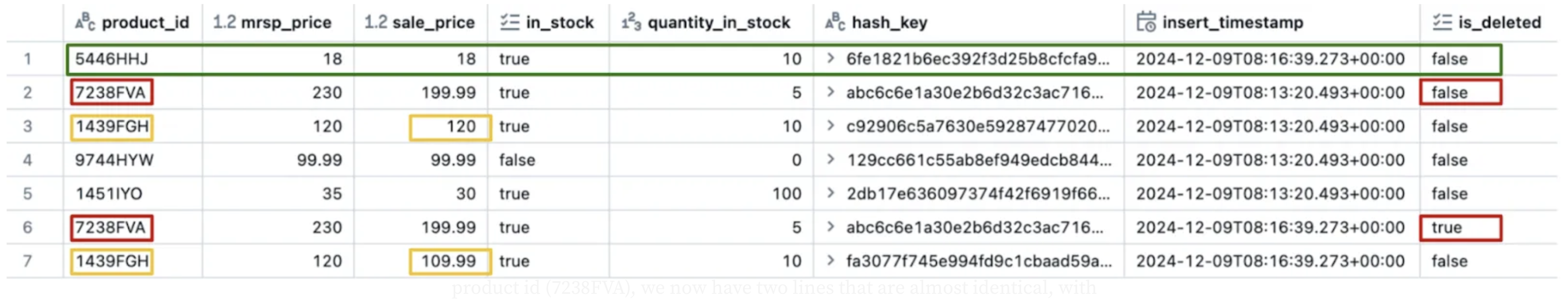
The raw table now contains 7 rows, 4 with the old (first) timestamp and 3 with the new timestamp. This is expected since 2 product ids (1451IYO, 9744HYW) never changed, so we had no updates for them in the second. For product id (7238FVA), we now have two lines that are almost identical, with the difference being that in the one with the latest timestamp the is_deleted field is now true, signifying a logical deletion. Furthermore, we have 1 row for the new product id (5446HHJ) that did not exist at (t0). Finally, the product id (1439FGH) has also two rows in the raw table. The distinguishing factor between them is a change in the sale_price value, reflecting an update. Everything makes sense!

Current_schema_table_name:

In the “current” table we can observe that it contains 4 rows. 2 with the “old” insert_timestamp (1451IYO, 9744HYW) and the other two (1439FGH,5446HHJ) with the “new” one. This is also expected. The first two were not affected by the ingestion_pipeline and the latter two are the insert and the update. The deleted product does not exist in this table, as it has been logically marked as deleted.

History_schema_table_name:

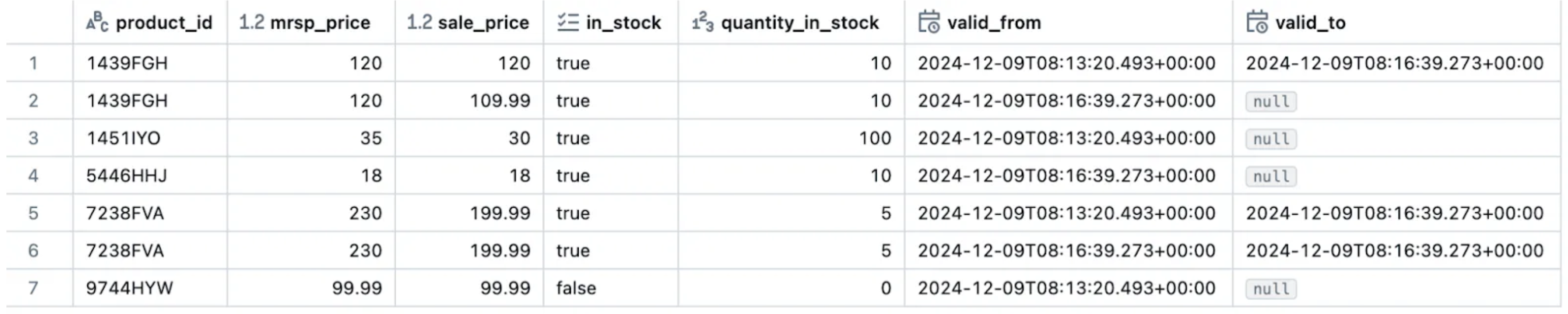
Now, in the “history” table you can easily identify all the products as well as all of their versions and the timestamps where it was active via the “valid_from” and “valid_to” fields.

It is worth noticing that the proposal above is for demonstration purposes. For a production pipeline there are many extra features that are needed. We should write code to ensure that the fields that come are always the same, and if there is an extra field we should take care of it so that the pipeline never fails and that the ingestion runs smoothly. Another point of consideration is to make sure that no duplicate records are coming in and if that is the case, we must deal with it accordingly. We should also perform quality checks, use an ingestion monitoring table to keep track and monitor our ingestions. Last but not least we should exploit the usage of the Databricks workflows in order to set our ingestion in a job and run it whenever it is necessary. There are also other things that we should take into consideration but they are out of scope for this blog.

Advantages of the proposed solution

To sum up the proposed solution is definitely the only way to go. The important thing to keep is that we capture the history in the raw data (bronze) and then the current and history tables that are built on top are a bit conceptual and based on the requirements. In addition we strongly recommend the insert only strategy that we followed in order to build our history. By following this strategy, the ingestion pipeline can focus on quickly appending raw data without worrying about all the rest aspects. The proposed implementation has the following advantages:

• Reproducibility and Platform Independence: The code is designed to be easily reproducible and not tied to a specific platform. Apart from reading and writing tables in Databricks, the remaining code can be executed on any environment that supports PySpark.
• Scalability: This solution is well-suited for Big Data. In real-world scenarios, where ingestion pipelines handle large volumes of data and run frequently, the execution time remains stable and efficient, regardless of the data size.
• Efficiency: By separating tables, the ingestion pipeline can focus solely on appending raw data, while analytical queries on the current and historical data remain unaffected. This ensures faster ingestion and better resource utilisation.
• Flexibility: Teams can directly access either the “current” table for up-to-date data or the “history” table for detailed historical analysis, bypassing the need to interact with the “raw” table. This simplifies workflows and improves performance.
• Data Transformation and Integrity: Transformations and enhancements can be applied to the current and history tables independently, leaving the raw data untouched. This ensures a consistent and unaltered source of truth while allowing tailored modifications downstream.
• Robustness: The implementation is designed to handle complex and large-scale ingestion pipelines reliably, ensuring consistent performance and adaptability to changing requirements.

In conclusion, building and maintaining data history is essential for ensuring accurate, compliant, and actionable insights from your data over time. By understanding and implementing techniques like Slowly Changing Dimensions (SCD) and leveraging powerful platforms such as Databricks, we can design scalable, efficient systems that track changes, preserve data integrity, and support decision-making processes. The proposed custom strategy provides a flexible and robust solution tailored to high-volume data environments, offering the benefits of clear data segmentation and efficient ingestion pipelines. However, you need to keep in mind that this solution was proposed based on our requirements and if those differ, another solution could be more suitable. As organisations continue to rely on data-driven decisions, having a strong foundation for data history will be key to unlocking the full potential of your data and driving business success.